Got a tip for us?
Let us know
Become a MacRumors Supporter for $50/year with no ads, ability to filter front page stories, and private forums.
Number '09 Question
- Thread starter sindekit
- Start date
- Sort by reaction score
You are using an out of date browser. It may not display this or other websites correctly.
You should upgrade or use an alternative browser.
You should upgrade or use an alternative browser.
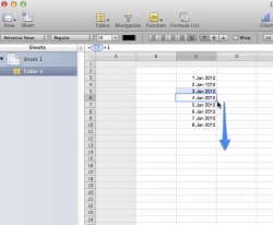
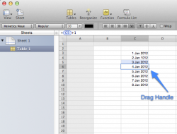
Assuming you want to increment the data by the same amount each time, say one day then you could put the current date in the top cell in the column, then the next cell underneath for the next date, put a formula that references the cell above +1 - See the screenshot below. If you then mouse over the bottom right hand corner of the cell, you will see a drag handle, drag this down each day and it will copy the formula down, incrementing the date by +1.
Hopefully you can see the formula in cell C6, = C5 +1

Hope that helps.
Hopefully you can see the formula in cell C6, = C5 +1

Hope that helps.
Last edited:
Assuming you want to increment the data by the same amount each time, say one day then you could put the current date in the top cell in the column, then the next cell underneath for the next date, put a formula that references the cell above +1 - See the screenshot below. If you then mouse over the bottom left hand corner of the cell, you will see a drag handle, drag this down each day and it will copy the formula down, incrementing the date by +1.
Hopefully you can see the formula in cell C6, = C5 +1
View attachment 325472
Hope that helps.
I think you mean the bottom right corner of the cell to see the drag handle.
Assuming you want to increment the data by the same amount each time, say one day then you could put the current date in the top cell in the column, then the next cell underneath for the next date, put a formula that references the cell above +1 - See the screenshot below. If you then mouse over the bottom left hand corner of the cell, you will see a drag handle, drag this down each day and it will copy the formula down, incrementing the date by +1.
You don't even have to do that much. Just enter the first date, and pull down the drag handle on the bottom right hand corner of the cell. It will correctly guess that you want to increment the date by 1 for each cell.
I think you mean the bottom right corner of the cell to see the drag handle.
yes, you are right thanks for the correction.
----------
You don't even have to do that much. Just enter the first date, and pull down the drag handle on the bottom right hand corner of the cell. It will correctly guess that you want to increment the date by 1 for each cell.
Now that is strange, I thought that would work as well, but when I tried it last night it just repeated the date sequence, rather than extend it. Tried it again today and it works as you suggested. I know Excel is pretty clever when it comes to extending date ranges and I initially thought that Numbers was not going to do what I needed. Thanks for the comment.
I need further help now:
I decided that I wanted to include another column for %loss. I figured out the formula to calculate it right, but I want to know if I could make it so it rounds up to the nearest hundredth place? Cause right now, it shows numbers like "1.43129770992366" . Oh and how do I make it so that my % column won't be included in the graph or if possible I can make it so that it has it's own graph?
Either way would be fine.
Thanks in advance.
I need further help now:
I decided that I wanted to include another column for %loss. I figured out the formula to calculate it right, but I want to know if I could make it so it rounds up to the nearest hundredth place? Cause right now, it shows numbers like "1.43129770992366" . Oh and how do I make it so that my % column won't be included in the graph or if possible I can make it so that it has it's own graph?
Either way would be fine.
Thanks in advance.
In Excel, you would do a formula like this: =Round(formula,2). That would round you to 2 decimal places. Going down in number gets you closer to the decimal and negative puts you across to the other side (-2 would round to the nearest hundred). The opposite is true also.
I haven't tried this in Numbers but don't see why it should be different.
I need further help now:
I decided that I wanted to include another column for %loss. I figured out the formula to calculate it right, but I want to know if I could make it so it rounds up to the nearest hundredth place? Cause right now, it shows numbers like "1.43129770992366" . Oh and how do I make it so that my % column won't be included in the graph or if possible I can make it so that it has it's own graph?
Either way would be fine.
Thanks in advance.
If you are just concerned with the display, on the View menu select "Show Format Bar", select the cells, and on the format bar you can set % format and set the number of digits. Without the format bar, but with the Toolbar, bring up the Inspector and you can set the format from there.
There doesn't seem to be a way to remove data from a graph. At least for me the Delete key does nothing even though it appears to be active. You can create a graph for any selection of data. I suggest using the built-in help since there are quite a few things you can do.
Register on MacRumors! This sidebar will go away, and you'll see fewer ads.


