Two Excel questions

[Smileyguy]

Hi folks,

I'm working on a fairly big spreadsheet of data on the mileage and carbon emissions of cars (It contains data on pretty much every car on the market here in Ireland, so it's pretty hefty). I need to do two things, and I'm wondering if Excel is up to the task.

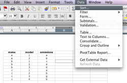
1. Currently the data is organised in a simple list alphabetically by car brand. However, I need to create a second list ranking the cars from the lowest emissions to the highest. The emission figures are in column G - is there a function I can use to automatically do this?

I presume there is a solution to the above, the real reason for starting this thread though is the following....

2. Based on its carbon emissions, every car in Ireland is assigned a 'carbon rating' of A, B, C, D, E or G, with A representing the most efficient and G representing the least. Each of these ratings corresponds to a particular rate of motor tax.

For example:

A = less than 120 grams of carbon per kilometre = €100 annual motor tax
B = 121-140 grams of carbon per kilometre = €150 annual motor tax

I have a column with an A-G figure for every car, but I also need to set up another column with the figure for motor tax beside it. Is there any way to do this automatically without going through thousands of cars and doing it manually?

I hope my questions were clear-ish. Thanks in advance for any help...

 

[NAG]

1. Select the columns you need to organize (all your data set).

Data (menu) > Sort (menu item) > Select the primary column to organize by (emissions column) and then select the secondary (probably the name/maker column).

2. You can set up nested if then statements but you can only do up to 7. You can also set up a user defined function that uses cases instead but I'm not sure if 2008 supports that. You can then just fill down and all the references will auto fill.

 

[JNB]

First question: Data>Sort

 

[Smileyguy]

I've figured number 1 out no problem now, thanks a million guys.

If you have the time, could you or anybody else shed any more light on how to go about number two? I'm using Office X I should have mentioned.

Thanks very much.

 

[NAG]

Here is a tutorial.

NOTE: VBA support was dropped in Office 2008 (will probably be back in the next version of office though) so this method won't work if you upgrade to that version.

 

[GGJstudios]

1. You can sort by any column you like. Simply select the range to be sorted, then Data > Sort.

2. You can do nested IF statements, but if you have a large number of possibilities, it's better to to a =VLOOKUP with a table.

 

[swiftaw]

Two ways:

1. Use the IF function, nested a few times.

If(ratingcell="A", tax for A, IF(ratingcell="B", tax for B, IF(ratingcell="C", tax for C, IF(ratingcell="D", tax for D, IF(ratingcell="E", tax for E, tax for G)

2. Use a lookup table, then the LOOKUP function
away from the main data, create two columns, one containing the letter A,B,C,D,E,G, one containing the corresponding tax value. Then, in the cell for each car, use the LOOKUP function. =LOOKUP(cell containing emission rating for current car, cells containing ratings in lookup table, cells containing taxes in lookup table)

 

[Smileyguy]

Okay, I've been trying the second problem using the LOOKUP solution suggested. I've created a simple A-G table with the corresponding tax values separate to the main data, and have used the function suggested by swiftaw:

=LOOKUP(cell containing emission rating for current car, cells containing ratings in lookup table, cells containing taxes in lookup table)

However, the problem I'm having is that for these three data values, I need the first to fill down as I do, but the second two to remain constant. As it stands, all three values automatically fill down, which means I can only use the function for six rows at a time.

Thanks for all the help - this has been really useful

 

[swiftaw]

Okay, I've been trying the second problem using the LOOKUP solution suggested. I've created a simple A-G table with the corresponding tax values separate to the main data, and have used the function suggested by swiftaw:

=LOOKUP(cell containing emission rating for current car, cells containing ratings in lookup table, cells containing taxes in lookup table)

However, the problem I'm having is that for these three data values, I need the first to fill down as I do, but the second two to remain constant. As it stands, all three values automatically fill down, which means I can only use the function for six rows at a time.

Thanks for all the help - this has been really useful

Suppose that your lookup table is containd in the columns AA and AB, rows 1 thru 6.

Suppose your rating for each car is stored in column D, and tax in column E, starting with row 2 and moving on down.

So for cell E2. the entry would be =LOOKUP(D2, $AA$1:$AA$6, $AB$1:$AB$6)

If you copy and past this down column E everything should work, the first entry (D2) would change to D3, D4, D5, etc as needed, but the other entries would remain fixed.

 

[Smileyguy]

Beautiful, thanks a zillion. This has saved me lots of time.

It's been years since I've need to use Excel with any depth. I

 

[NAG]

To setup a constant use $ symbol eg $A$1 sets the constant to column A row 1 (ie it will always reference cell A1 no matter what way you fill).

 

[Smileyguy]

It works beautifully. Thanks so much.


Out of curiosity, can Numbers do all this stuff?

One last quick question: Is it possible to use the LOOKUP function with ranges of values?

For example, let's say I hadn't manually assigned each car an A to G rating based on its emissions, and I wanted to do this with LOOKUP. Lettered ratings correspond to emissions as follows:

< 120g per kilometre: A
120g-140g per kilometre: B
121g-155g per kilometre: C
156g-170g per kilometre: D

and so on...

Could I do this automatically? I've tried setting up a LOOKUP table where one column has the different ranges of emissions, and the other has the letters. I've tried representing the ranges as either 121:140 and 121...140, but neither has worked.

It's not too important, but I'd be keen to know if there's a way to do this.

 

[logana]

One last quick question: Is it possible to use the LOOKUP function with tables of values?

Could I do this automatically? I've tried setting up a LOOKUP table where one column has the different ranges of emissions, and the other has the letters. I've tried representing the ranges as either 121:140 and 121...140, but neither has worked.

It's not too important, but I'd be keen to know if there's a way to do this.

Yes - you have to set up the table so the values go from lowest at the top to highest at the bottom - but don't use ranges use the highest number in the range eg 120,140,155 etc and then Excel will look down the lookup table until it finds the number that is not lower than itself (if you follow - if the value is 139 it will go down the table as far as the 140 value and then pickup the value in the cell next to it in the table - that's the normal way to arrange the table).

Great fun !!

 

[Consultant]

If you are doing such work, you should take some courses. Even a basic, inexpensive class from community college covers all these and more.

 

[NAG]

To answer the Numbers question, Numbers can do this (and in a similar way too, uses the same conventions).

Numbers isn't quite as good as Excel for graphing though (little rough as well as no support for error bars).