Combining duplicate entries in '08 Excel

[chrisf79]

I am a real novice with excel and this may be a novice's question but it's driving me nuts!

BACKGROUND
(I am starting an excel file that contains text from 18th to 21st century cookbooks. Once complete I will be able to track how frequently certain word are used as well as how words come into and out of fashion ('eel,' 'ambergris,' 'fry,' 'spam,' etc)

QUESTION:
As I add data from specific texts I am pasting onto the bottom of my "words" column (A), with the corresponding frequency in B. I then alpha the whole document, insert a new B column. Repeat. Repeat. Repeat. Subsequently, I have dozens of duplicates in my A column (e.g. 'about' or 'the') but the word frequency is correct in the other columns.
I want to delete duplicate entries in my 'A' column while keeping their frequency in the column that refers to the specific text (which increases to the left as I add entries)


Any and all advice would be great!

Best,

Chris...

 

[James_C]

Hi Chris, this is pretty easy to do with Pivot Tables, which will summarise the data in the table for you. It will add multiple instances of the repeated words and sum the frequency, and give you a nice summarised table.

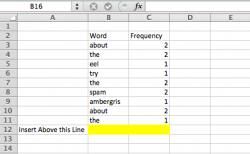
To create a pivot table make sure that you have a heading directly above your first line of data, and at the bottom highlight in yellow the first blank row at the bottom of your table. This is to remind you insert data between the last row of data and the highlighted rows. As we are going to create a named range for the data, so that as you add more data to the table the named range will be updated as well.

See the screenshot below of how the source data table should look



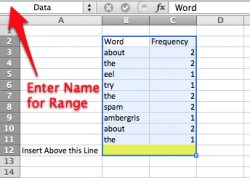
Ok we need to define a name for your data. Select the entire table including the heading and the blank row at the bottom of the table (the one highlighted in yellow). Click on the Name Range box, just above Col A as shown below, and enter a suitable name, I used 'Data'.



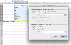
Now we are going to create the pivot table, I am using Excel 2011, but you can use 2008, although I am a little rusty on how it used to work, but I am sure you can work it out if I am a little off. From the Data menu choose Pivot Table (Might be called something slightly different in 2008 Pivot Table Wizard or something). Then in the Dialog where it asks you for a range enter the name of the range 'Data'.



I think from memory 2008 has a step by step wizard that may then ask you if you want to create on a separate sheet or on the same sheet. I find it easier to create on a separate sheet.

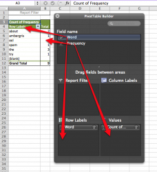
Ok the next part in 2008, it is a bit different from 2011, and you will be presented with a grid for the pivot table, you need to drag the Word (names) to the Row Labels and the frequency to 'values'.



Hopefully you will see a summarised table similar to the above.

When you add more date you need to insert data into the source data table between the last row and the first blank row. Just insert the number of blank rows that you need if you are typing this in manually. That way the named range 'Data' will automatically expand. To check that this is correctly picking up all the data you can click on the named range/ cell box enter 'Data' and it will show you the named range.

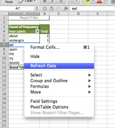
You will need to refresh the pivot table to get it to update as you add new data. Right click on the pivot table and choose refresh.



I hope that helps - Note you are not deleting the duplicated rows in the source table, but you can copy and paste as values the pivot table to have a nice summary of your word count.

Hope this helps.

 

[chrisf79]

James,

Thank you so much for the detailed information!...

Unfortunately, it doesn't seem so be working for me.
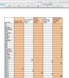
Here is a screen grab of the actual table:



As you can see I have multiple columns of texts and a master column of words.

I've followed, I think, your very clear instructions. but when I make the pivot table I end up with something like this...


(For some reason the dialogue box can't be screen grabbed.)

As I enter the data something into the box something is obviously wrong with either how I am putting in the data or something. All I get is a couple '1' entries here and there and it gets more screwy as I enter more data.

I'll keep plugging away at it.
Thanks again so much for your generous response.

 

[chrisf79]

James,

I actually just got the pivot table to sort of work.
I can make the table for one text but I cannot enter data for more than one without the table getting all screwy.
I'll post an update if things progress.

C.

 

[James_C]

Hi Chris, sorry for the delay in replying. Now I see your source data I can see the problem. You need to get your data into a format that works better with Pivot Tables. The problem is you have multiple columns for data that you want to sum (the different books). You need to do one of the following

1. Add a total column that sums the total number of word counts over all the books. If Column F was the last column then add a column in Column H called 'Word Total' and have a formula that sums Columns B to F and copy it all the way down to the bottom of the table. I know this may appear odd as each line may only be summing one value, but we want to have just one Column for the frequency in the pivot table. The Copy and paste as values the first column AAAWord and the Total column to a separate tab on the spreadsheet and build the pivot table from that. The downside to this is, it is not so easy to see the books that are driving the final results and you will have to recreate the summary table each time you add additional data.

EDIT - Actually you don't need to create a separate table - you just need to add the total column to the value part of the pivot table, and ignore the individual book columns (but you will need to select the entire table range when first creating the pivot table). This is probably easier than recreating the data table in 2 below, although the suggestion in 2 is a neater approach.

or

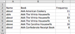
2. Create a table that has the data in the format

Three Columns

Word Name , Name of Book, Frequency

It will not take long to build from your data. Just copy the first column (names) to a new sheet into Col A, then paste the name of the first book AAA American Cookery (1798) into the second column, from the first line down to the last row of names that you have in Col A, then paste the frequency values in from Col B for the first book into Column C. Now sort this new table by Frequency and delete all the rows with nothing in Col C.

Move to the bottom of the table and repeat the process for all the other books.

You will end up with a table that looks a little like this



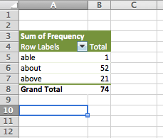
Then when you create a pivot table it will hopefully give you the result that you want



If you use this approach you can double click on a pivot table result value and Excel will create a new tab with the source data, so you can easily see the books that are generating the data.



I am sure you may have already solved your problem, but hopefully this will help for the future.