Specific Search in spreadsheet

[GerritV]

Hello,

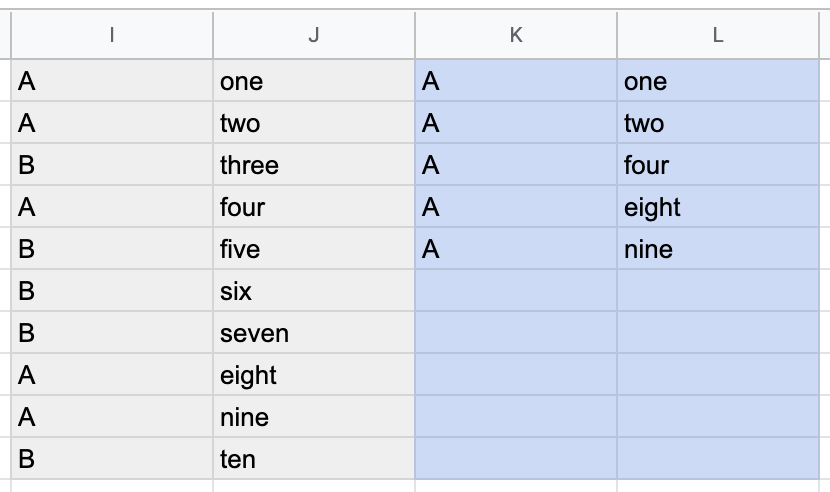
Say I have a number of data in columns I-J.
I is an index, J is a text.
What I want is to search all lines that have "A" in column I, and have the adjacent text from column J to appear in column L, while skipping the lines that have "B".
Anyone knows a formula for this that I can enter in column L ?
I wouldn't mind the intermediate column K.

 

[liya1201]

A quick thought: could you select column I and J and "sort" column I alphabetically?

 

[GerritV]

A quick thought: could you select column I and J and "sort" column I alphabetically?

Thanks for the suggestion.
I'll elaborate a little more. This is a shared google spreadsheet, and when I perform any sort action on a tab, the others will see it the same way. So I was thinking of creating a second tab where there's some triage going on for one team member only. I hope I'm clear enough here.

 

[Moakesy]

This will work in Excel, but I don't know Google well enough to be sure if it will work in there.

Copy and paste the formula below, paste it into cell 'L1', then copy it down into all those cells I've shown in green. Put the letter 'A' in cell K1 (as highlighted yellow in my example). If you change the value in cell K1, then the results change.

=IFERROR(INDEX($J$1:$J$10,SMALL(IF(K$1=$I$1:$I$10,ROW($I$1:$I$10)- MIN(ROW($I$1:$I$10))+1,""), ROW())),"")

 

[Moakesy]

Or thinking about it, if Google Docs does pivot tables, you could just create one of those. Much simpler!!

 

[GerritV]

This will work in Excel, but I don't know Google well enough to be sure if it will work in there.

Copy and paste the formula below, paste it into cell 'L1', then copy it down into all those cells I've shown in green. Put the letter 'A' in cell K1 (as highlighted yellow in my example). If you change the value in cell K1, then the results change.

=IFERROR(INDEX($J$1:$J$10,SMALL(IF(K$1=$I$1:$I$10,ROW($I$1:$I$10)- MIN(ROW($I$1:$I$10))+1,""), ROW())),"")

Wow, thanks for this formula!
I managed to translate it to Dutch, and so far I get "ONE" in cell L1. After copying down, the other cells in column L remain empty. And when I type "B" in cell K1, column L is empty as well.
I'll hopefully figure it out.
[doublepost=1563605264][/doublepost]

Or thinking about it, if Google Docs does pivot tables, you could just create one of those. Much simpler!!

Agree, but I thought a pivot table doesn't like empty cells in it's reach (which I have a lot of).

 

[Moakesy]

Try putting “A” in cell K2,K3 etc, as you may have accidentally deleted a $ sign during translation.

I’m trying to work out why changing the value in K1 doesn’t work. A common reason is because there is a ‘space’ there. So the cell entry is ‘B’+space or space+B instead. The easiest way to check is to use the formula =LEN(cell ref). This counts the number of characters in the cell. So B is one character, but B+space will be two characters.